Game Theory

In every society, people interact all the time. Sometimes, those interactions are cooperative, and other times, they are competitive. In either case, the term interdependence applies—one person's behaviour affects another person's well-being, either positively or negatively.

As you know, Web3 is mostly about incentives. Most specifically, it's about aligning incentives. To do that, calculating the costs of attacks, or determining whether the tokenomics we are designing are accurate enough, we need Game Theory.

We will define this discipline as a method of studying strategic situations — everything that constitutes imperfect competition is a strategic setting.

tip

A situation is strategic if the outcomes that affect you depend on actions not just of yourself but also of others.

Game theory is useful in many ways, as it defines a language with which we can converse and exchange ideas. And it provides a framework that guides us in constructing models of strategic settings and traces through the logical implications of assumptions about behaviour.

During this part of the onboarding, we are going to dive deep into Game Theory. As an overview, you will learn about what exactly is a game, dominant strategies, best responses, modelling tools (such as Cournot and Stackelberg), how to deal with mixed strategies, the role of evolution on decisions, how to deal with sequential games and how the information we have affects the outcome of games.

Most importantly, you will learn that life is a game, and having the tools to cope with that is amazing.

info

If this is your first time hearing about Game Theory, we recommend you to see https://oyc.yale.edu/economics/econ-159/lecture-1

What is a game, exactly?

In short, games are formal descriptions of strategic settings. So, game theory is a methodology of formally studying situations of interdependence — formally, because we use mathematically precise and logically consistent structures. Every game can be described by four components:

1. Players: Decision-makers in the scenario (e.g., two firms, two politicians, or two classmates).
2. Actions/Strategies: Each player's options (e.g., set a price, vote for a policy, choose a number).

Payoffs Are Central. To figure out the "best" move, we need to know what each player is trying to achieve. Without payoffs—some sense of objectives (self-interest, collective good, moral satisfaction)—we can't analyze the situation properly.

An extensive‐form game is essentially a game tree that shows players' moves step by step, in the order they're made, including what each player knows when making a decision. We will have:

• Nodes – These are "decision points" in the game. You start with an initial node (the first decision in the game) and move along branches as players take actions.
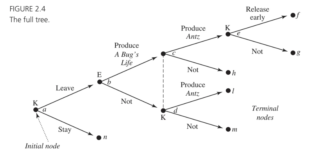
• Branches (Actions) – From each node, the possible moves are shown as branches. In the example below, the node labeled with "K," for instance, means it's Katzenberg's turn; each outgoing branch from that node is one of his possible actions.

• Terminal Nodes – When no further choices remain, you arrive at terminal nodes, each corresponding to an outcome with specific payoffs (or "utilities") for each player. These payoffs represent each player's preference ranking over outcomes.

• Information Sets – If a player doesn't know exactly which node they're at (because they don't see the other player's choice yet), then these nodes are grouped together by a dashed line (an "information set"). This indicates imperfect information—the player makes the same decision at any node in that information set.

An extensive‐form game is essentially a game tree that shows players' moves step by step, in the order they're made, including what each player knows when making a decision. We will have:

Let's think the following example: two players, Katzenberg (DreamWorks) and Eisner (Disney), are deciding whether to produce the bug‐themed animated films (Antz vs. A Bug's Life). Initially, Katzenberg can either stay at Disney or leave to form DreamWorks. That choice kicks off the game.

J. Watson. Strategy: An Introduction to Game Theory, Norton 2002

The Normal Form

Here, the most important concept is the notion of a strategy.

tip

A strategy is a complete contingent plan for a player in the game — a full specification of a player's behaviour, which describes the actions that the player would take at each of his possible decision points.

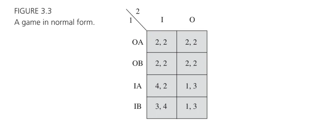
A normal‐form (or "strategic‐form") game is just a more compact way of describing all the players' moves and payoffs—without drawing the tree. Here, we will have:

1. Complete Contingent Plans: each player's strategy must specify what they'll do at every decision point or information set they control (even if that point might never be reached). For example. given three possible decisions in a extensive form, the normal-form strategy has to say: "If I'm at node $a$, I do $X$; If I'm at $c$ or $d$, I do $Y$; and if I'm at $e$, I do $Z.$"
2. Strategy Sets: For each player $i$, we list all possible strategies (i.e. all possible ways they could behave across every decision point). We label this set as $S_i$.
3. Strategy Profiles and Payoffs: A strategy profile is one specific choice of strategy for each player $(s_1, s_2, \dots, s_n)$. Once everyone's strategies are fixed, we know exactly which outcome —terminal node— is reached. That outcome determines the players' payoffs. Formally, each player $i$ has a payoff function $u_i : S \rightarrow \R$, where $S = S_1 \times S_2 \times \dots S_n = \prod_{i=1}^{n} S_i$. This means that for any strategy profile $s \in S$, $u_i(s)$ gives player $i$'s payoff.
4. Matrix Representation (Two-Player Case): When both players have a finite set of strategies, we can draw a matrix:
   • Rows = strategies of player 1,
   • Columns = strategies of player 2,
   • Each cell = payoff pair (one payoff for each player)

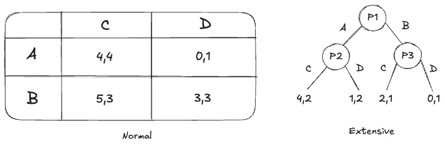
Essentially, the normal form is a big list (or matrix) of complete plans for every player, along with the payoff outcomes for each combination of those plans. It's the same information as the extensive form, just boiled down to strategies and payoffs.

Here there is an example:

One way of viewing the normal form is that it models a situation in which players simultaneously and independently select complete contingent plans for an extensive-form game.

Classic Games

The Prisoner's Dilemma

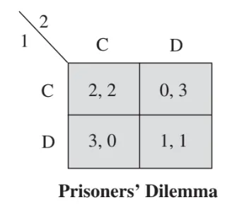
Two prisoners are arrested and interrogated separately. Each must choose to Cooperate (C) with the other (stay silent) or Defect (D) (confess).

• If they both cooperate, they both get a moderate penalty.
• If one defects while the other cooperates, the defector goes free and the cooperator gets the worst outcome.
• If both defect, each gets a lesser sentence than if only one had squealed, but worse than if both had cooperate.

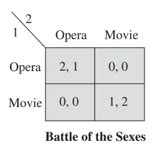
Battle of the Sexes

Two friends want to meet up but must each independently choose between two events: Opera (O) or Movie (M). Both prefer being together over being apart, but they differ on which event they like more: Player 1 prefers Opera, Player 2 prefers Movie.

• If they pick different events, they get nothing (they're alone).
• If they pick the same event, they meet, and each is happier if it's the event they personally like more.

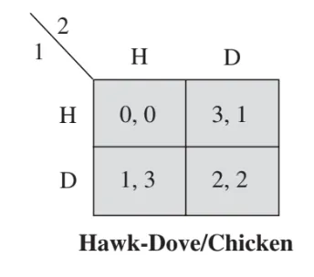
The chicken problem

Two drivers speed toward each other. Each must choose either to Hold course (H) or Swerve (S):

• If both swerve, neither "wins" big, but both avoid the terrible crash.
• If one holds and the other swerves, the holder is seen as "tough" (higher payoff), and the swerver is the "chicken."
• If both hold, they crash—a very bad payoff for both.

Dominant and Weakly Dominant Strategies

When looking at a game in normal form, it's often helpful to check if any player has a dominant strategy, or if any strategy is dominated:

• A strictly dominant strategy is one that yields a strictly higher payoff than any other choice no matter what the opponent does. If you find one, it's automatically your best move—no guesswork needed.
• A strictly dominated strategy is one that always gives a strictly lower payoff than some other strategy, again regardless of the opponent's action. You can safely discard any strictly dominated strategy, because there's always a strictly better choice available.

Sometimes we look at weakly dominant/dominated strategies, meaning the payoff is at least as good in all cases and strictly better in at least one. These are less forceful than "strictly," but still guide player choices.

As we seen before, in the Prisoner's Dilemma, each prisoner must either Cooperate (C) or Defect (D). Here, D is a strictly dominant strategy for each player:

• If your partner chooses C, choosing D gets you 3 instead of 2.
• If your partner chooses D, choosing D gets you 1 instead of 0.
• So D always pays strictly more.

Consequently, C is strictly dominated: you always do worse by cooperating. Ironically, this leads to both prisoners choosing D and ending up at $(1,1)$, which is worse for them collectively than $(2,2)$ would have been if they'd both cooperated.

tip

Never play a strictly dominated strategy, since there is another strategy that always does better.

Nash Equilibrium

Now that we understand dominant and dominated strategies, we can introduce one of the most important concepts in game theory: Nash equilibrium. It is a strategy profile where no player has an incentive to unilaterally change their strategy. In other words, given what the other player is doing, each player is making the best possible choice they can.

Formally, a strategy profile $(s_1^*, s_2^*, \dots, s_n^*)$ is a Nash equilibrium if, for every player $i$: $u_i(s_i^*, s_{-i}^*) \geq u_i(s_i, s_{-i})$ for all possible alternative strategies $s_i$. This means that no single player can switch to a different strategy and improve their payoff while the other players' strategies remain unchanged. Now, let's see how Nash equilibrium appears in the classic games we've discussed.

For example, in the Chicken Game, if both Swerve $(S,S)$, they avoid the crash but don't gain dominance. Then, if one Holds while the other Swerves $(H,S)$ or $(S,H)$, the Holder wins, and the Swerving player loses face. Lastly, if both Hold $(H,H)$, they crash, which is the worst outcome.

For finding the Nash equilibrium, lets analyze two scenarios:

• If Player 1 Holds, Player 2's best response is to Swerve, because $0 > -1$.
• If Player 1 Swerves, Player 2's best response is to Hold, because $2 > 1$.

This means there are two Nash equilibria: $(H,S)$ and $(S,H)$. So, the game represents a brinkmanship situation—neither player wants to Swerve, but if neither backs down, they both lose badly. This is why Chicken is a model for real-world conflicts where compromise is needed to avoid disaster.

Iterative Elimination

Now that we understand dominant and dominated strategies as well as the Nash equilibrium, we introduce a useful technique for simplifying games: Iterative Elimination of Dominated Strategies. This method helps us systematically remove strategies that are clearly bad choices, making it easier to find rational outcomes—sometimes leading directly to the Nash equilibrium.

In many games, some strategies are strictly worse than others, regardless of what the other player(s) do. When a strategy is strictly dominated, we can eliminate it because a rational player will never choose it. After eliminating one bad strategy, others may become strictly dominated as well—so we iterate the process until no more dominated strategies remain. The steps for eliminate would be:

1. Identify and remove any strictly dominated strategies.
2. Update the game and check if new strategies have become strictly dominated.
3. Repeat until no more strictly dominated strategies exist.
4. Analyze the remaining game to find the likely outcome.

For example, in the Prisoner's Dilemma we can see that:

• For Player 1: Comparing (C) and (D):
  • If Player 2 plays C, Player 1 prefers D (3 > 2).
  • If Player 2 plays D, Player 1 still prefers D (1 > 0).
  • So, D strictly dominates C for Player 1—we eliminate C.
• For Player 2: Same logic applies—D strictly dominates C, so C is eliminated.

After eliminating C for both players, we are left with only (D, D)—which we already identified as the Nash equilibrium.

So, in the Prisoner's Dilemma, iterative elimination leads us straight to the Nash equilibrium. The process confirms that both players will defect, even though $(C, C)$ would have been better for both.

Common knowledge vs. Mutual knowledge

So far, we've explored how players rationally choose strategies based on the available information. But what if we need to reason about what others know—or even what others know about what we know? This is where the distinction between mutual knowledge and common knowledge becomes important.

• Mutual Knowledge: You and I may each know there is a pink hat in the room, but I might not know if you know I have seen it.
• Common Knowledge: Extends infinitely: "I know X; you know X; I know that you know X; you know that I know that you know X; etc."

The difference can be subtle but crucial. Many strategic behaviors (coordinating on a single pass to defend, or driving all guesses down to 1 in the two-thirds game) rely not just on rationality but on everyone knowing that everyone knows (and so forth) the logical structure of the game. Some key insights to keep in mind are:

1. Mutual knowledge is not always enough for coordination.
   • If two soccer players mutually know they should defend against a pass, they still might not execute properly if they aren't sure the other will react accordingly.
2. Common knowledge enables deeper reasoning.
   • In games like the two-thirds guessing game, where players must predict how others will think, the reasoning process involves assumptions about what everyone knows about what everyone knows.
3. Expectations of rationality rely on common knowledge.
   • Nash equilibrium assumes that players are rational and know that others are rational—but if this rationality is only mutual knowledge (not common knowledge), uncertainty might still influence decisions.

Best Response Analysis

Some games cannot be resolved purely through deleting dominated strategies. Sometimes no strategy is outright dominated, yet players still have sensible moves once they consider beliefs about what the other side will do. This leads to the concept of a best response.

A best response is a strategy that maximizes a player's payoff given a belief about what the other players will do. Formally, a strategy $s_i^*$ is a best response to the other players' strategies $s_{-i}$ if it provides at least as high a payoff as any alternative choice would, assuming the other players stick to $s_{-i}$. In many games, no single strategy dominates all others, so we look for which option is best once we have a guess (or belief) about the opponents' moves.

Example: Soccer Penalty Kicks

• Players: The shooter (kicker) versus the goalkeeper.
• Strategies: The kicker chooses left, middle, or right; the goalkeeper dives left or right (ignoring the "stay put" possibility for simplicity).
• Payoffs: The kicker's probability of scoring vs. the goalkeeper's probability of saving (the two payoffs add to zero).

Key Observation: Although each side wants to outguess the other, we can systematically check which kicking direction is optimal given beliefs about how often the goalkeeper dives left or right.

Eliminating Never-Best-Responses

• In a simplified matrix, kicking to the middle never yielded the highest expected payoff for any belief about the goalie's moves, so "middle" is never a best response.
• The lesson generalizes: never play a strategy that is not a best response against any possible belief about your opponent.

In actual soccer, further considerations (accuracy, the possibility of kicking high or low, a goalkeeper staying still) complicate the analysis. Nevertheless, the idea of ruling out moves that are never optimal for any forecast of the opponent remains an important principle.

Example: Partnership and Effort Levels

• Players: Two partners jointly owning a firm or collaborating on a project.
• Strategies: Each partner chooses an effort level $S_1$ or $S_2$ in the interval $[0,4]$
• Profit Function: $4(S_1+S_2)+B \times S_1 \times S_2$, shared 50-50 by the two players.
• Payoffs: Each partner's payoff is half the total profit minus the square of their own effort, capturing disutility from working harder.

Now, we want to find the best response. Because each partner's action is a real number (continuosly from 0 to 4), we use calculus:

1. Fix the other partner's effort $S_2$
2. Maximize Player 1's payoff with respect $S_1$
3. The first-order condition (derivate = 0) yields a best-response function $\hat{S}_1 = 1 + B \times S_2$
4. By simmetry, $\hat{S}_2 = 1 + B \times S_1$

Iterative Elimination

• If certain effort levels are never best responses for any action by the partner (e.g., very high or very low hours), they can be ruled out.
• Re-checking which responses remain valid once those strategies are removed can further shrink the set of plausible choices.
• Eventually, this process converges to a single pair $(S_1^*, S_2^*)$, found by solving the system: $S_1^* = 1 + B \times S_2^*$, $S_2^*= 1 + B \times S_1^*$
• Symmetry implies $S_1^* = S_2^*$ and simple algebra gives $S_1^* = S_2^* = \frac{1}{1-B}$

Efficiency and Externalities

At this solution, each partner individually chooses less than the socially optimal effort. The reason is an externality: each person's extra effort raises total profit, but half of that benefit goes to the other partner. Because each partner only captures half of the added gains from their own effort, each exerts too little effort relative to the cooperative optimum.

Cournot Duopoly

Cournot Duopoly is a classic model in economics that illustrates how two firms, each producing the same good, compete by choosing quantities rather than prices. It bridges two extreme cases covered in introductory economics: perfect competition (many firms, each a price-taker) and pure monopoly (a single firm). Cournot thus helps analyze imperfect competition—a situation more common to real-world markets.

Model Details

• Players: Two firms (Firm 1 and Firm 2).
• Strategies: Each firm $i$ chooses a quantity $q_i$ of an identical product.
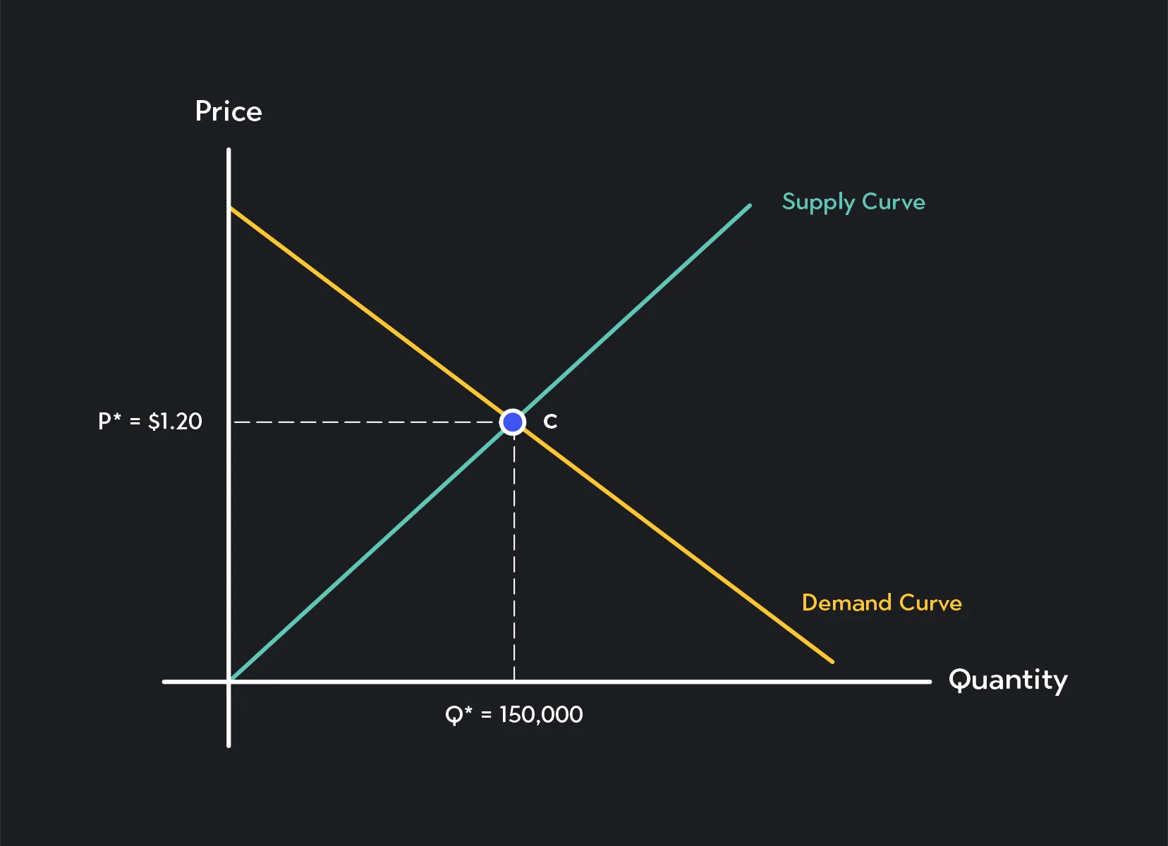
• Demand & Price: Market price depends on total quantity $q_1 + q_2$. For simplicity, assume a linear demand curve $P = a - b(q_1 \times q_2)$ where $a,b > 0$

• Costs: Each firm has constant marginal cost $c$ per unit, so producing $q_i$ units costs $c \times q_i$.
• Payoffs: Firm $i$'s profit is $\pi_i = P \times q_i - c \times q_i = [a - b(q_1 + q_2)]q_i - c \times q_i$

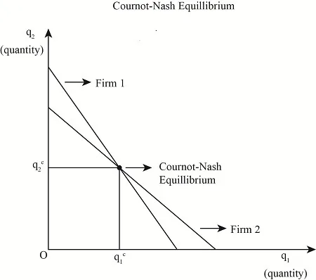
In this case, for finding the Nash equilibrium you will need to find the best-response functions, where each firm chooses $q_i$ to maximize its own profit, taking the other firm's output as given. By setting the first derivative of $\pi_i$ w.r.t. $q_i$ to zero, one obtains:

$q_1^*= \frac{a-c}{2b}-\frac{1}{2}\times q_2$ and $q_2^* = \frac{a-c}{2b}-\frac{1}{2}\times q_1$

The Cournot Nash Equilibrium occurs where these best-response lines intersect. Since the game is symmetric, $q_1 = q_2$. Solving yields: $q_1^* = q_2^* = \frac{a-c}{3b}$.

Monopoly vs. Competition

A monopolist (a single seller) producing alone would choose the monopoly quantity, $\frac{a-c}{b}$. Then, under perfect competition with constant marginal cost $c$, total industry output would reach $\frac{a-c}{b}$. While Cournot total output $2 \times \frac{a-c}{3b}$ is higher than the monopoly output, but lower than the competitive output, the corollary of this is that:

• Price under Cournot is between the monopoly price and the competitive price.
• Profits for each firm are less than under monopoly but greater than under perfect competition. Consumers pay less than the monopoly price but more than the fully competitive price.

Some observations are that the two firms could theoretically produce the smaller monopoly quantity and enjoy higher combined profits, but each has a private incentive to cheat by increasing output beyond the agreed limit. Actual collusion is also illegal in many places. Also, because one firm's larger output depresses price for both, each firm responds by reducing its own quantity. The actions are strategic substitutes.

Stackelberg Competition and Backward Induction

So far, we've analyzed games using normal-form representations (payoff matrices) and extensive-form representations (game trees). Now, we shift our focus to dynamic games, where players make decisions sequentially rather than simultaneously.

One famous example of this kind of game is the Stackelberg duopoly, which demonstrates how firms compete in a market when one firm moves first and the other responds.

In a Stackelberg duopoly, two firms compete in a market by choosing quantities of a product to produce. However, unlike in the Cournot model (where firms choose simultaneously), the Stackelberg model assumes:

1. Firm 1 (The leader) moves first, choosing its quantity $q_1$.
2. Firm 2 (The follower) observes $q_1$ and then chooses $q_2$.

Since the follower reacts to the leader's decision, Firm 1 can anticipate Firm 2's best response and use this to maximize its own profit.

The Problem of Credible vs. Incredible Threats

Imagine that Firm 2 threatens to produce a very high quantity if Firm 1 enters the market, making it unprofitable for Firm 1. This is similar to how an incumbent firm might threaten a price war to deter a new entrant.

However, once Firm 1 actually enters the market, Firm 2 must reconsider: does it really make sense to produce an excessively high quantity (or start a price war)?

The answer is usually no—Firm 2, once faced with the actual situation, will likely choose a more rational response instead. This is an example of an incredible threat—a statement that seems rational in advance but isn't actually believable when the decision has to be made.

Backward induction

To analyze games where players move sequentially, we use backward induction, a method that starts from the end of the game and works backward to determine the optimal strategy for each player.

How Backward Induction Works

1. Look at the last decision in the game tree: At this stage, the player only needs to pick the best option from a set of final choices.
2. Eliminate suboptimal actions: Remove choices that wouldn't be rational for that player.
3. Move backward to earlier decision nodes: Now, the previous player can anticipate how the later player will respond and adjust their own decision accordingly.
4. Repeat until you reach the first move: This process determines the optimal path through the game.

Example: Market Entry with a Price War Threat

Imagine a potential entrant (Firm 1) considering entering a market dominated by an incumbent (Firm 2). The game works as follows:

• Firm 1 chooses whether to Enter (E) or Stay Out (O).
• If Firm 1 Stays Out (O), the game ends, and Firm 2 enjoys a monopoly.
• If Firm 1 Enters (E), then Firm 2 chooses whether to Fight (F) by starting a price war or Accommodate (A) by allowing competition.

Firm 1 / Firm 2	Accommodate	Flight
Enter	(Modest profit, modest profit)	(Loss, loss)
Stay Out	(0, Monopoly profit)	N/A

If we want to use backward induction:

• Firm 2's decision (last move):
  • If Firm 1 enters, Firm 2 can fight (leading to losses for both) or accommodate (leading to modest profits).
  • Clearly, fighting is irrational, since it results in losses.
  • So, if entry occurs, Firm 2's best move is to accommodate.
• Firm 1's decision (first move):
  • Firm 1 anticipates that Firm 2 will not actually fight, even if it threatens to.
  • So, Firm 1 should enter the market, knowing that Firm 2 will eventually accommodate.

Backward Induction in Stackelberg Competition

In a Stackelberg duopoly, Firm 1 (the leader) knows Firm 2 will react optimally to its decision. Instead of guessing how much to produce, Firm 1 anticipates Firm 2's response and chooses its own production level accordingly.

1. Firm 2's Reaction Function: Given any $q_1$ from Firm 1, Firm 2 maximizes its profit by producing $q_2$ based on $q_1$.

   This results in a function $q_2 = s_2(q_1)$, describing how Firm 2 reacts to any $q_1$.

2. Firm 1 Anticipates and Maximizes Profit: Knowing that Firm 2 follows $s_2(q_1)$, Firm 1 chooses $q_1$ strategically to maximize its own profit.

   This gives Firm 1 a first-mover advantage—it can manipulate Firm 2's decision to gain a higher profit than in simultaneous-move Cournot competition.

tip

Stackelberg competition demonstrates first-mover advantage, where the leader chooses its strategy knowing the follower will react optimally.

The Candidate-Voter Model

In many political science models, we assume there are two candidates in an election who freely pick their positions on the ideological spectrum. By contrast, the candidate–voter model fixes each candidate's position in advance. Specifically, we consider a setting in which every voter could be a potential candidate, and each has a known "true" stance on a political spectrum (e.g., left or right). Voters will vote for whichever candidate is closest to them, ideologically.

A first lesson from such a model is that there can be multiple Nash Equilibria in which different subsets of the population run for office. Some equilibria might have candidates relatively close together; others might have them far apart. Moreover, not all equilibria end up "crowded at the center"—a contrast to simpler median-voter models.

A second lesson is that entry by an additional candidate on one side of the spectrum can end up benefiting the other side, because the entering candidate "splits" the votes on his or her own ideological side. In other words, a left-leaning candidate who enters might pull votes away from a more moderate left candidate, inadvertently helping the right-leaning candidate to win.

Example: Dating

To show how multiple equilibria (including inefficient ones) can arise, consider a simpler scenario: a pair of individuals attempting to meet but forgetting to communicate which activity they prefer. Suppose they have two date options—say, going apple-picking or seeing a play. Each has a favorite activity, yet they both prefer to meet rather than to miss each other. In pure-strategy equilibrium, they might coordinate on one activity (both choose apple-picking, or both choose the play). However, one also finds a mixed-strategy Nash Equilibrium in which each person randomizes over the two options—and thus fails to meet a significant fraction of the time.

Although that mixed equilibrium is inefficient (they would be happier always meeting), it remains a valid outcome if neither side can unilaterally do better. Hence, mixed strategies in such coordination settings can produce suboptimal outcomes in practice.

Three Interpretations of Mixed Strategies

When we say a player (or candidate) "mixes" across strategies, there are at least three ways to interpret it:

1. Literal Randomization: The individual may actually toss a coin (or use some random device) to choose which move to make, as often suggested in sports or security contexts (e.g., "mixing up" pitches in baseball, or random checks in airport security).
2. Beliefs of the Opponent: A mixed strategy can represent the probability distribution that the opponent believes you are using. You might not literally randomize, but if others hold that belief, it can still produce equilibrium outcomes akin to random play.
3. Population Proportions: In a large population, the fraction (say, 30%) of people who adopt one strategy and the fraction (70%) who adopt another can be viewed as a "mixed" profile for society overall. Instead of each person individually randomizing, there is a stable split across the population.

Evolutionarily Stable Strategy

A formal concept, Evolutionarily Stable Strategy (ESS), was introduced by biologist John Maynard Smith in the 1970s. Informally, a strategy $S$ in a large population is called evolutionarily stable if no small group of mutants adopting some alternative $S'$ can successfully invade and displace $S$.

• If a mutation does worse on average than $S$ when both are mostly playing against $S$, it dies out.
• If the mutation does as well versus $S$ as $S$ does against itself, but fails in mutant-vs-mutant encounters, it also dies out.

In both cases, the incumbent strategy $S$ remains dominant.

If we take a Prisoner's dilemma example, when everyone cooperates (C), defectors (D) easily invade because $D$ does better against $C$. So $C$ is not stable. Conversely, if everyone is defecting, a lone cooperator cannot improve its payoff, so defection is stable in that model.

Thus, we see how purely self-regarding payoffs can lead to "nature" locking in an outcome like universal defection—highlighting that evolutionary outcomes need not be "good" or "efficient."

Strict Dominance, Nash Equilibrium, and ES

Further analysis shows:

• Strictly Dominated strategies cannot be stable: a strictly dominating strategy will always invade.
• If a strategy $S$ is not a Nash best response to itself, then it cannot be evolutionarily stable. (Any profitable unilateral deviation—some $S'$—forms a successful mutation.)

However, not every Nash strategy is stable. If $S$ is merely a weak best response to itself, it might be invaded by a mutation that does equally well versus $S$ but better when facing itself. A strict Nash strategy, on the other hand, is guaranteed to be evolutionarily stable in these simplified asexual models.

Imperfect Information

So far, we've focused on games where players know exactly where they are in the game tree when making decisions. However, real-world strategic situations often involve imperfect information, where players lack complete knowledge about past actions. This distinction is crucial for understanding subgame perfect equilibrium (SPE) and how it refines Nash equilibrium.

Perfect vs. Imperfect Information

• A game has perfect information if, at every decision node, the player on the move knows all previous actions taken by other players.
• A game has imperfect information if a player, when making a decision, does not know exactly which node they are at in the game tree.

In extensive-form games, imperfect information is represented using information sets, which group together nodes that a player cannot distinguish between. The key feature of an imperfect information game is that a player must choose a strategy without knowing all past moves.

Example: Market Entry with Hidden Pricing Strategy

Imagine a potential entrant (Firm 1) considering entering a market where an incumbent (Firm 2) has already set prices, but the entrant doesn't know whether the incumbent is aggressive or passive.

• If the incumbent's pricing strategy is hidden, Firm 1 must make a decision without knowing whether it is facing an aggressive or accommodating competitor.
• This uncertainty groups multiple decision nodes into an information set—Firm 1 cannot distinguish between facing an aggressive or passive incumbent.

tip

Imperfect information games introduce strategic uncertainty befcause players must act without knowing the full history of the game.

Subgame Perfect Equilibrium

While Nash equilibrium is a powerful tool, it has a limitation:

• Some Nash equilibria rely on "incredible threats"—strategies that seem rational on paper but wouldn't actually be followed through in real-time play.
• Subgame perfection eliminates these unrealistic Nash equilibria by ensuring that strategies remain rational at every stage of the game.

A Subgame Perfect Nash Equilibrium (SPE) is a refinement of Nash equilibrium that requires that the chosen strategy must be a Nash equilibrium in every subgame of the original game.

More formally, a subgame is a smaller game that starts at a specific decision node and includes all its successors without crossing an information set boundary.

• If a node and all its successors form a well-defined game tree, it is a subgame.
• If a node is part of an information set with other nodes, it does not initiate a subgame (because the player doesn't know which node they are at).

Example: Market Entry Game (Revisited)

Let's return to our market entry game, where Firm 1 decides whether to Enter (E) or Stay Out (O), and if Firm 1 enters, Firm 2 decides whether to Fight (F) or Accommodate (A).

1. If Firm 1 Stays Out, Firm 2 gets its monopoly profit.
2. If Firm 1 Enters, Firm 2 can either:
   • Fight, leading to losses for both.
   • Accommodate, allowing competition with modest profits.

Using Nash equilibrium, we might initially consider a strategy where Firm 2 threatens to fight in order to scare Firm 1 away. But is this credible?

Identifying Subgames

• The entire game is a subgame.
• The subgame that starts after Firm 1 enters is another subgame.

Applying Subgame Perfection

• If we analyze only the subgame starting from "Enter", Firm 2 should choose Accommodate because fighting is irrational—it hurts Firm 2 too.
• Knowing this, Firm 1 should ignore the threat of a price war and confidently enter.

The subgame perfect equilibrium is (Enter, Accomodate), eliminating the unrealistic thret of a price war.

tip

The key here is that SPE refines Nash equilibrium by ensuring strategies remain rational in every subgame, removing "incredible threats".

So… how can we use this for research?

To illustrate how game theory can provide structured insights, let's analyze a real-world example of attack feasibility and incentives for price manipulation within a lending protocol. The protocol relies on oracles like Chainlink or Uniswap TWAP for price feeds. This problem can be framed as a strategic interaction between players with conflicting objectives.

Define the Players

At its core, the model involves three main players:

1. The attacker, who attempts to manipulate the oracle price to extract profit.
2. The oracle nodes, responsible for validating price data.
3. The lending protocol, which enforces liquidation rules and manages systemic risk.

Identify the Strategies

• The attacker decides whether to manipulate the price feed or refrain.
• Oracle nodes can report honest or manipulated prices. Nodes face penalties for misreporting.
• The protocol determines monitoring mechanisms and penalties to disincentivize manipulation.

Outline the Payoffs

The payoffs reflect the costs and benefits associated with each strategy:

• For the attacker: $\text{Profit=Inflated Gains−Manipulation Cost}$

• The attacker's goal is to ensure the expected value remains positive.

  $\text{Profit} = \text{Inflated Gains} - \text{Manipulation Cost} > 0$

• For oracle nodes:Honest reporting earns rewards, while misreporting incurs penalties. $\text{Net Payoff} = \text{Reward} - \text{Penalty (if dishonest)}$

• For the protocol: The protocol's payoff is linked to minimizing risks, where equilibrium occurs when manipulation becomes prohibitively expensive.

Analyzing Equilibrium

Using Nash Equilibrium, the system stabilizes when no player can unilaterally improve their payoff by deviating. In this case:

• Attackers cease manipulation when the cost of attack exceeds the benefit.
• Oracle nodes report honestly when the expected penalty for misreporting outweighs the rewards of collusion.

For Uniswap's TWAP oracle, the cost of manipulation depends on the liquidity of the pool and the duration required to influence the price:

$C_{\text{manipulation}} \approx \Delta P \cdot L \cdot T$

• $\Delta P$: The price change resulting from manipulation.
• $L$: Liquidity in the pool.
• $T$: Time period for the TWAP calculation.

For Chainlink, which relies on decentralized oracle nodes, the attack cost scales linearly with the number of compromised sources:

$C_{\text{Chainlink}} \approx f \cdot C_{\text{per-source}}$

• $f$: The fraction of oracle nodes an attacker needs to corrupt.
• $C_{\text{per-source}}$: The cost to compromise a single oracle.

Key Insights for Protocol Design

By modeling the problem mathematically, the analysis reveals actionable insights:

1. Raising the Cost of Manipulation: Increasing pool liquidity (L) or extending TWAP duration (T) reduces the feasibility of attacks.
2. Incentivizing Honest Oracle Behavior: Designing significant penalties for misreporting ensures that honest reporting becomes the dominant strategy.
3. Decentralization as a Defense: For Chainlink-like systems, increasing the number of nodes (f) exponentially raises the cost of successful attacks.

Resources

https://oyc.yale.edu/economics/econ-159 — Recommended if interested! Most of these notes are taken from this course.

https://www.youtube.com/watch?v=PsLaI4jDftA&pp=ygUSR2FtZSB0aGVvcnkgY291cnNl

A. Dixit and B. Nalebuff. Thinking Strategically, Norton 1991

J. Watson. Strategy: An Introduction to Game Theory, Norton 2002

P.K. Dutta. Strategies and Games: Theory And Practice, MIT 1999